
일단 라이브러리들을 불러오고, 'train.csv', 'test.csv' 파일 또한 불러오자.
import pandas as pd
import numpy as np

train = pd.read_csv('train.csv')
test = pd.read_csv('test.csv')
그 후 제대로 파일을 불러왔는지 train.head()로 확인해보았다.
train.head()
| 1 | 0 | 3 | Braund, Mr. Owen Harris | male | 22.0 | 1 | 0 | A/5 21171 | 7.2500 | NaN | S |
| 2 | 1 | 1 | Cumings, Mrs. John Bradley (Florence Briggs Th... | female | 38.0 | 1 | 0 | PC 17599 | 71.2833 | C85 | C |
| 3 | 1 | 3 | Heikkinen, Miss. Laina | female | 26.0 | 0 | 0 | STON/O2. 3101282 | 7.9250 | NaN | S |
| 4 | 1 | 1 | Futrelle, Mrs. Jacques Heath (Lily May Peel) | female | 35.0 | 1 | 0 | 113803 | 53.1000 | C123 | S |
| 5 | 0 | 3 | Allen, Mr. William Henry | male | 35.0 | 0 | 0 | 373450 | 8.0500 | NaN | S |
위의 데이터 프레임을 살펴보면 승객 데이터에서 제공되는 특성은 10가지가 있는데,
- Survived: 타깃입니다. 0은 생존하지 못한 것이고 1은 생존을 의미합니다.
- Pclass: 승객 등급. 1, 2, 3등석.
- Name, Sex, Age: 이름 그대로 의미입니다.
- SibSp: 함께 탑승한 형제, 배우자의 수.
- Parch: 함께 탑승한 자녀, 부모의 수.
- Ticket: 티켓 아이디
- Fare: 티켓 요금 (파운드)
- Cabin: 객실 번호
- Embarked: 승객이 탑승한 곳. C(Cherbourg), Q(Queenstown), S(Southampton)
그 중에서 의미를 바로 알기 힘든 것들을 자세하게 살펴봤다.
- Survivied - 생존 여부(0은 사망, 1은 생존; train 데이터에서만 제공)
- Pclass - 사회경제적 지위(1에 가까울 수록 높음)
- SipSp - 배우자나 형제 자매 명 수의 총 합
- Parch - 부모 자식 명 수의 총 합
그리고 Survived 특성을 참고하여 차트를 확인하면
import seaborn as sns
import matplotlib.pyplot as plt
f, ax=plt.subplots(1, 2, figsize=(12,6))
train['Survived'].value_counts().plot.pie(explode=[0,0.1],autopct='%1.1f%%',ax=ax[0],shadow=True)
ax[0].set_title('Survived')
ax[0].set_ylabel('')

# 이제 이렇게쓰면 안됨
# sns.countplot('Survived',data=train,ax=ax[1])

# 대신 이렇게 수정하면 됨
sns.countplot(x='Survived',data=train)

ax[1].set_title('Survived')
plt.show()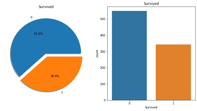
위에 설명한 것처럼 0은 사망, 1은 생존을 의미하니까 탑승객의 60% 이상이 사망했다는 결론을 얻을 수 있다.
우선 타이타닉호 사건에 대해서 찾아봤는데 등급(Pclass)이 높을수록
그리고 여성과 아이를 먼저 구조했거 때문에 Survived는 당연히 타깃으로 잡고, (Pclass, Sex, Age)를 특성 기준으로 삼으면 좋을 것 같다.
한번 성별과 나이, Pclass까지 참고하여 차트를 확인해 보자.
f,ax=plt.subplots(1,2,figsize=(12,6))
train['Survived'][train['Sex']=='male'].value_counts().plot.pie(explode=[0,0.1],autopct='%1.1f%%',ax=ax[0],shadow=True)
train['Survived'][train['Sex']=='female'].value_counts().plot.pie(explode=[0,0.1],autopct='%1.1f%%',ax=ax[1],shadow=True)
ax[0].set_title('Survived (male)')
ax[1].set_title('Survived (female)')
plt.show()
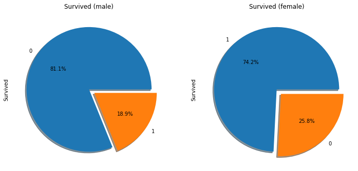
위에서 말했듯 여성과 아이를 먼저 구하는 문화가 있었기 때문에 여성이 생존율이 높은것을 확인 할 수 있다.
밑에 있는 차트는 Pclass와 (Sex, Survived)특성을 비교한다.
pd.crosstab([train['Sex'],train['Survived']],[train['Pclass']],margins=True).style.background_gradient(cmap='summer_r')
| 3 | 6 | 72 | 81 |
| 91 | 70 | 72 | 233 |
| 77 | 91 | 300 | 468 |
| 45 | 17 | 47 | 109 |
| 216 | 184 | 491 | 891 |
보다시피 높은 등급일수록 생존 확률이 높았다는 것을 확인할 수 있다.
특히 3등급 객실에 있었던 남성의 경우 생존률이 엄청 낮은 것을 확인할 수 있다.
누락 데이터 확인
train.info()
RangeIndex: 891 entries, 0 to 890
Data columns (total 12 columns):
 #   Column       Non-Null Count  Dtype
---  ------       --------------  -----
 0   PassengerId  891 non-null    int64
 1   Survived     891 non-null    int64
 2   Pclass       891 non-null    int64
 3   Name         891 non-null    object
 4   Sex          891 non-null    object
 5   Age          714 non-null    float64
 6   SibSp        891 non-null    int64
 7   Parch        891 non-null    int64
 8   Ticket       891 non-null    object
 9   Fare         891 non-null    float64
 10  Cabin        204 non-null    object
 11  Embarked     889 non-null    object
dtypes: float64(2), int64(5), object(5)
memory usage: 83.7+ KB
Age가 null값이 있는 것을 확인할 수 있다.
아까 특성을 정할 때 중요하게 생각한다고 한 만큼 지우는것보다 중간 나이로 넣는 방식으로 해보자.
train['Age'][train.isnull().any(axis=1)]
0      22.0
2      26.0
4      35.0
5       NaN
7       2.0
       ...
884    25.0
885    39.0
886    27.0
888     NaN
890    32.0
Name: Age, Length: 708, dtype: float64median = train["Age"].median()
train["Age"].fillna(median, inplace=True)
중간 값을 넣고 다시 수치를 확인하면
train.info()
RangeIndex: 891 entries, 0 to 890
Data columns (total 12 columns):
 #   Column       Non-Null Count  Dtype
---  ------       --------------  -----
 0   PassengerId  891 non-null    int64
 1   Survived     891 non-null    int64
 2   Pclass       891 non-null    int64
 3   Name         891 non-null    object
 4   Sex          891 non-null    object
 5   Age          891 non-null    float64
 6   SibSp        891 non-null    int64
 7   Parch        891 non-null    int64
 8   Ticket       891 non-null    object
 9   Fare         891 non-null    float64
 10  Cabin        204 non-null    object
 11  Embarked     889 non-null    object
dtypes: float64(2), int64(5), object(5)
memory usage: 83.7+ KB
"Age" 특성에 null이 사라져서 누락된 값이 채워진 것을 볼 수 있다.
또한 "Sex" 특성에 있는 "male", "female"을 수치형으로 바꾼다.
i = 0
while i < len(train["Sex"]):
  if train["Sex"][i] == "male" :
    train["Sex"][i] = 0
  else :
    train["Sex"][i] = 1
  i += 1
train["Sex"]
0      0
1      1
2      1
3      1
4      0
      ..
886    0
887    1
888    1
889    0
890    0
Name: Sex, Length: 891, dtype: object
마찬가지로 "Age" 특성에 아이(12살 이하)와 어른을 구별하기 위해 두개의 범위를 만든다.
i = 0
while i < len(train["Age"]):
  if train["Age"][i] < 13.0 :
    train["Age"][i] = 0.0
  else :
    train["Age"][i] = 1.0
  i += 1
train["Age"]
0      1.0
1      1.0
2      1.0
3      1.0
4      1.0
      ...
886    1.0
887    1.0
888    1.0
889    1.0
890    1.0
Name: Age, Length: 891, dtype: float64
여기서 한번 예측 모델을 실행하고 결과를 도출해보자.
from sklearn.tree import DecisionTreeClassifier
from sklearn.model_selection import train_test_split
from sklearn import metrics #accuracy measure

train_df, test_df = train_test_split(train, test_size=0.3,random_state=0)
target_col = ['Pclass', 'Sex', 'Age']
train_X=train_df[target_col]
train_Y=train_df['Survived']
test_X=test_df[target_col]
test_Y=test_df['Survived']

features_one = train_X.values
target = train_Y.values

tree_model = DecisionTreeClassifier()
tree_model.fit(features_one, target)
dt_prediction = tree_model.predict(test_X)

print(metrics.accuracy_score(dt_prediction, test_Y))
0.7947761194029851
예측 모델은 0.7947761194029851이라는 결과가 나온다.
test 값에도 적용하기 위해 test.csv의 "Sex", "Age" 특성에도 똑같이 처리를 해주고 다시 실행하고 파일을 만들어서 제출을 해보자.
i = 0
while i < len(test["Sex"]):
  if test["Sex"][i] == "male" :
    test["Sex"][i] = 0
  else :
    test["Sex"][i] = 1
  i += 1
test["Sex"]
0      0
1      1
2      0
3      0
4      1
      ..
413    0
414    1
415    0
416    0
417    0
Name: Sex, Length: 418, dtype: objecti = 0
while i < len(test["Age"]):
if test["Age"][i] < 13.0 :
test["Age"][i] = 0.0
else :
test["Age"][i] = 1.0
i += 1
test["Age"]
0      1.0
1      1.0
2      1.0
3      1.0
4      1.0
      ...
413    1.0
414    1.0
415    1.0
416    1.0
417    1.0
Name: Age, Length: 418, dtype: float64
밑은 결과 제출을 위해 예측모델 파일을 생성하는 코드이다.
# predict test data with pre-trained tree model
test_features = test[target_col].values
dt_prediction_result = tree_model.predict(test_features)

# Create a data frame with two columns: PassengerId & Survived. Survived contains your predictions
PassengerId = np.array(test["PassengerId"]).astype(int)
dt_solution = pd.DataFrame(dt_prediction_result, PassengerId, columns = ["Survived"])

# Write your solution to a csv file with the name my_solution.csv
dt_solution.to_csv("my_solution_one.csv", index_label = ["PassengerId"])
제출 후 결과 확인

그닥 점수는 높지는 않다. 특성을 많이 안 건드렸기 때문 ㅎ0ㅎ
요약
캐글(Kaggle) 타이타닉 경진대회(competition) 참가
타이타닉의 데이터셋을 전처리하여 Survived 특성과 연계해 생존자를 더 잘 구분할 수 있게 해야한다.
- 훈련세트와 테스트 셋으로 구분되어 있는 데이터셋 다운로드 후 파일을 확인한다.
- 의미를 알기 힘든 특성은 자세하게 살펴보면 설명을 찾을 수 있었다.
- 그리고 타이타닉호 사건에 대해 살펴보았는데, 여성과 아이를 먼저 구조했고, 승객 등급에 따라 방의 위치가 달랐기 때문에 Pclass, Sex, Age, Survived 4가지 특성을 이용하였다.
- Sex 특성의 경우 female과 male 처럼 되어있기 때문에 수치형으로 바꿔주었다.
- Age 특성의 경우 누락 데이터는 중간 값을 넣어 진행시켰고 아이와 어른을 구분하기 위해 12살 이하라는 범위를 만들어 특성을 변환하였다.
- 그렇게 예측값은 약 79%가 나왔다. 95%정도가 완벽한 예측 정도라고 추정하자면 대략 16%정도가 부족한데, 특성 값에서 비싼 객실의 유무를 구분할 수 있는 티켓 요금(Fare)과 객실 번호(Cabin), 그리고 승객이 탑승한 곳(Embarked)와 같이 특성을 더 추가하고 확인하였으면 좋은 점수가 나오지 않았을까 싶다.
- 참고 문헌: 핸즈온 머신러닝
- Github link: 머신러닝 실습 3